최근에 저는 PoseTrack Dataset으로 실험을 진행해보고 있는데, video 데이터에서 어떻게 하면 pose estimation을 좀 더 잘 할 수 있을까 생각해보다가 Crowdpose: Efficient crowded scenes pose estimation and a new benchmark 를 읽어보게 되었습니다.
이 논문에서는 사람이 많은 영상 속에서 포즈를 잘 예측하기 위해 싱글 person 포즈 estimation에 joint candidate loss를 적용하고 global association 그래프 모델을 활용하여 joint candidate 중 맞는 joint를 골라 포즈를 estimation합니다.

먼저 일반 싱글 person pose estimation은 receptive fields 가 제한되어 crowd scene에서 좋은 성능을 내지 못합니다. 따라서 여기선 joint candidate을 활용하는데 i번째 사람의 proposal인 region Ri를 SPPE에 넣고 히트맵 pi를 뽑습니다. 이때, Ri는 i번째 사람에 속하는 joint와 속하지 않는 joint 두 가지 타입의 joint가 존재합니다.(이를 타겟 조인트와 interference joint라고 부르는데 여기서 interferencejoint는 다른 사람의 타겟 조인트 일수 있으므로 직접 제한을 걸진 않고 다른 강도를 줘서 출력하게 됩니다.)
i번 사람의 조인트에 대해 타겟 조인트 히트맵 $T^k_i$를 만들고 간섭 조인트에 대해서도 히트맵 $C^k_i$를 만듭니다. 이후 최종 loss를 이렇게 정의하는데 뮤는 실험시(cross vali을 통해) 0.5로 정했다고 합니다.

이후 이 joint candidate 중 실제 joint 를 추출하기 위해 person joint graph 를 활용합니다. Joint node는 P1와 p2사이의 거리가 해당 조인트의 히트맵의 u1 u2 즉 가우시안 response 크기의 최소값에 deviation을 곱한 값보다 작다는 조건을 만족하면 같은 조인트를 예측하는 그룹으로 만듭니다. 이 그룹을 한개 조인트 노드로 만들어 휴먼 디텍터에 의해 생긴 사람 노드에 후보 joint들의 response score (아마 히트맵 score일듯)로 weight를 주어 연결합니다.
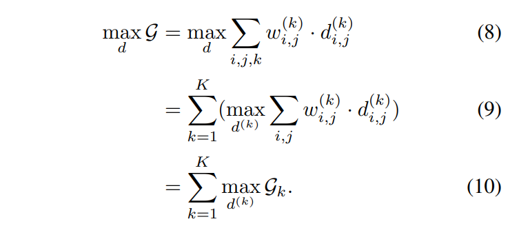
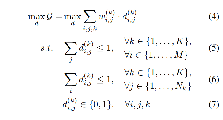
이 그래프를 푸는 것은 각 엣지의 weight들의 합을 maximize하는 것인데, 이는 각 종류별 조인트의 weight를 최대화 하는 문제로 decompose 할 수 있습니다.
논문 요약
Joint-Candidates SPPE(single person pose estimator)
Loss Design
For the $i^{th}$ human proposal, we input its region $R_i$ into our SPPE network and get the output heatmap $P_i$. There are two types of joints in $R_i$, that is, the joints belong to the $i^{th}$ person, and the joints belong to other human instances (not the $i^{th}$ person). name them as target joints and interference joints respectively.
Our goal is to enhance target joints response and suppress interference joints response. However, we don’t suppress them directly since interference joints for the current proposal can be regarded as target joints for other proposals. Thus, we can leverage interference joints to estimate human poses with other human proposals in a global manner. Therefore, to utilize those two kinds of joint candidates, we output them with different intensities.
Heatmap Loss
For the $k^{th}$ joint in the $i^{th}$ person, we denote the target joint heatmap as $T^k_i$, consisting of a 2D Gaussian $G(p^k_i |σ)$, centered at the target joint location $p^k_i$, with standard deviation σ.
For interference 간섭 joints, we denote them as a set $Ω^k_i$. The heatmap of interference joints is denoted as $C^k_i$, consisting of a Gaussian mixture distribution $\Sigma_{p\inΩ^k_i}G(p|σ).$ Our proposed loss is defined as,

where µ is an attenuation 감쇠 factor ranged in [0,1]. As aforementioned, interference joints will be useful in indicating joints of other human instances. Therefore, we should consider it in a global view by cross-validation. Finally, we have µ = 0.5, which fits our intuition: interference joints should be attenuated but not over-suppressed. The conventional heatmap loss function can be regarded as our special case where µ = 0.
limit A conventional SPPE depends on a high-quality human detection result. Its tasks are locating and identifying target joints according to the given human proposal. If SPPE mistakes interference joints for target joints, it will be an unrecoverable error. Missing joints cannot be restored in the post-processing step like pose-NMS.
Person-Joint Graph
Due to our joint-candidate mechanism and redundant human proposals from human detector, joint candidates are numerically much greater than the actual joint numbers. To reduce redundant joints, we build a person-joint graph and apply a maximum person-joint matching algorithm to construct the final human poses
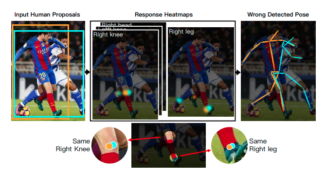
- fig 4. crowd scene ⇒ highly overlapped ⇒ tend to predict same actual joint. if we directly connect the highest response to build final poses, two human proposals will locate same right knee and right leg.
Joint Node Building
Since highly overlapped human proposals tend to predict the same actual joint (as Figure 4), we first group these candidates that represent the same actual joint as one joint node. Thanks to the high-quality joint prediction, candidate joints that indicate the same joint are always close to each other. Thus, we can group them using the following criterion: given two candidate joints located at $p^k_1$ and $p^k_2$ with control deviation $δ^k$, we label them as the same group, if

where $u^k_1$ and $u^k_2$ are the Gaussian response size of two joints on heatmaps, determined by the Gaussian response deviation. $δ^{(k)}$ is the parameter for controlling deviation of the $k^{th}$ joint, which we directly adopt from MSCOCO keypoint dataset [15]. The reason why we use $min\{u_1, u_2\}$ rather than a constant threshold is to guarantee that, only if $p_1$ and $p_2$ fall into each others’ control domain (radii are $u^k_1δ^k, u^k_2δ^k$) simultaneously, we group them together. One node represents a group of joints that cluster together by the above criterion. Now, by building a joint group as one node, we have joint node set J = {$v^k_j:$ for $k ∈ \{1, . . . , K\}, j ∈ \{1, . . . , N_k\}\}$, where $N_k$ is the number of joint nodes of body part k, $v^k_j$ is the $j^{th}$ node of body part k. The total number of joint nodes in J is $\Sigma_kN_k$.
Person Node Building
Person nodes represent the human proposals detected by human detector. We denote person node set as $H = \{h_i: ∀i ∈ \{1 . . . M\}\},$ where $h_i$ is the $i^{th}$ person node, and M is the number of detected human proposals. Ideally, a qualified human proposal tightly bounds a human instance. However, in crowded scenes, this condition is not always satisfied. The human detector will produce many redundant proposals, including truncated and incompact bounding boxes. We will eliminate these low-quality person nodes during global person-joint matching in Sec. 3.3.
Person-Joint Edge
After obtaining the node of both joints and persons, we connect them to construct our person-joint graph. For each person node $h_i$ , JC-SPPE will predict several candidate results of joints. If one of these candidates contributes to the joint node $v^k_j$, we build an edge $e^k_{i,j}$ between them. The weight of $e^k_{i,j}$ is the response score of that candidate joint, which is denoted as $w^k_{i,j}$. In this way, we can construct the edge set $E = \{e^k_{i,j} : ∀i, j, k\}$.
The person-joints graph can then be written as:

Globally Optimizing Association
goal - solving the above person-joint graph and maximizing the total edge weights.
Objective function as

where $d^{(k)}_{i,j}$ indicates whether we keep the edge $e^k_{i,j}$ in our final graph or not. The constraints of Eq. 5 and 6 enforce that each human proposal can only match at most one $k^{th}$ joint.
Note that G can be decomposed into K sub-graph $G_k =((H,J^{(k)}), E^{(k)})$, where $G_k$ is the sub-graph the only consist of the $k^{th}$ kind of joints. Thus, our objective function can be formulated as

As shown in Eq. 10, solving the global assignment problem in person-joint graph G is mathematically equivalent to solving its sub-graph Gk separately. Gk is a bipartite graph that composed of person subset and the $k^{th}$ joint subset. For each sub-graph, the updated Kuhn-Munkres algorithm [1] is applied to get the optimized result. By addressing each Gk respectively, we obtain the final result set R.
Given the graph matching result, if $d^{(k)}_{i,j} = 1$ the weighted center of $v^k_j$ is assigned to the $i^{th}$ human proposal as its k-th joint. Here, weighted center means the linear combination of candidate joints coordinate in $v^k_j$ and the weights are their heatmap response scores. In this way, the pose of each human proposal can be constructed. The person nodes that can not match any joint will be removed.
Computational Complexity
The inference speed of pose estimation is essential in many applications. We prove that our global association algorithm is as efficient as common greedy NMS algorithms. As the hereditary property identified by White and Whiteley [2], a graph G is $(k, l)−sparse$ if every nonempty sub-graph X has at most $k|X| − l$ edges, where $|X|$ is the number of vertices in sub-graph X and $0 ≤ l < 2k$. Consider the sub-graph $G^{(k)} = ((H,J^{(k)}), E^{(k)})$. It represents the connection between human proposals and the k-th type of joints. According to our statistics (Fig. 5), every human bounding box covers four persons at most in crowded scenes. Therefore, one person node builds connection edges to 4 joints at most. In other words, our personjoint sub-graph $G^{(k)}$ is (4, 0) − sparse since
Due to the sparsity of our person-joint graph, we can solve the association problem efficiently. We transform $E^{(k)}$ into an adjacency matrix $M_e^k$ (unconnected nodes refer to 0). According to the work of Carpaneto et al. [1], this linear assignment problem for the sparse matrix can be solved in $O(n^2)$, i.e., $O((|H| + |J^{(k)}|)^2)$. Since we have eliminated the redundant joints and there is a one-to-one correspondence between joints and persons, the expectation of $|J^{(k)}|$ is equal to $|H|$. Thus we have $O((|H| + |J^{(k)}|)^2) = O({|H|}^2)$. Such computation complexity is the same as the complexity of conventional greedy NMS algorithms.

- fig 5. Instance-Joint connection distribution. The x-axis denote the number of human bounding boxes that cover a same joint. This statistical result is based on the ground truth annotations.
Discussion
Our method adopts the graph-based approach to associate joints with human proposals in a globally optimal manner. Human proposals compete with each other for joint nodes. In this way, unqualified human proposals without dominant human instance would fail to be assigned any joints, since their joint response scores are all relatively low due to missing dominant human instance. Therefore, many redundant and poor human proposals are rejected. In comparison to our approach, conventional NMS is a greedy and instance-based algorithm, which is less effective. Although [10, 17, 27] proposed pose-NMS to utilize pose information, their algorithms are based on instances and cannot tackle the missing joints and wrong assembling problem. Our globally optimizing association method can deal with such situations well.
Dataset
Crowding Level Definition - need to define a Crowd Index first, which measure the crowding level in a given image. number of persons in an image seems to be a good measurement. However, the principal obstacle to solving crowded cases is not caused by the number of persons, but rather by occlusion in a crowd. Therefore, we need a new Crowd Index to indicate crowding level. In the bounding box of the i-th human instance, we denote the number of joints that belonging to the i-th person and other (not i-th) persons as $N^a_i$ and $N^b_i$ respectively. $N^b_i/N^a_i$ is the crowd ratio of the i-th human instance. Our Crowd Index is derived by averaging the crowd ratio of all persons in an image:

where n indicates the total number of persons in the image. We evaluate the Crowd Index distribution of three public benchmarks: MSCOCO (person subset), MPII and AI Challenger. As shown in Figure 6, uncrowded scenes dominate these benchmarks, which leads the SOTA methods only focus on these simple cases and ignore the crowded ones.
Experiments
- Crowd Index: easy (0-0.1), medium (0.1-0.8) and hard (0.8-1)
- human detector (YoloV3 [43])
- pose estimation network provided by AlphaPose
training step, we adopt rotation (±30), scaling (±30%) and flipping data augmentation.
- input resolution is 320 × 256 and the output heatmap resolution is 80 × 64.
- learning rate is set to 1 × 10⁻⁴ and 1 × 10⁻⁵ after 80 epochs.
- Mini-batch size is set to 64, and RMSprop [7] optimizer is used
testing, the detected human bounding boxes are first extended by 30% along both the height and width directions and then forwarded through the Joint-candidate SPPE
- two Nvidia 1080Ti GPUs
Ablation Studies
replace our joint-candidate loss with mean square loss ⇒ 66.0% to 61.7%


댓글